Accessing MT data from the NCI Geonetwork¶

For this example, we will access some of The University of Adelaide MT Data. To search for this, let’s visit the NCI GeoNetwork

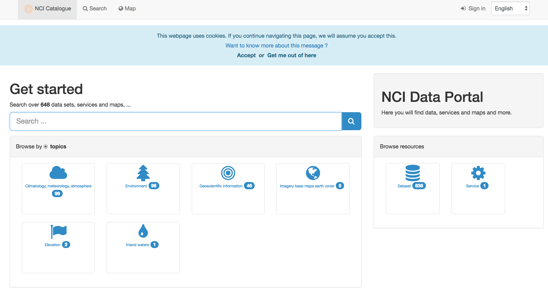
Let’s begin by searching using the keyword magnetotellurics:

Now click on The University of Adelaide Magnetotellurics Data.

This will bring you to The University of Adelaide MT data parent record:

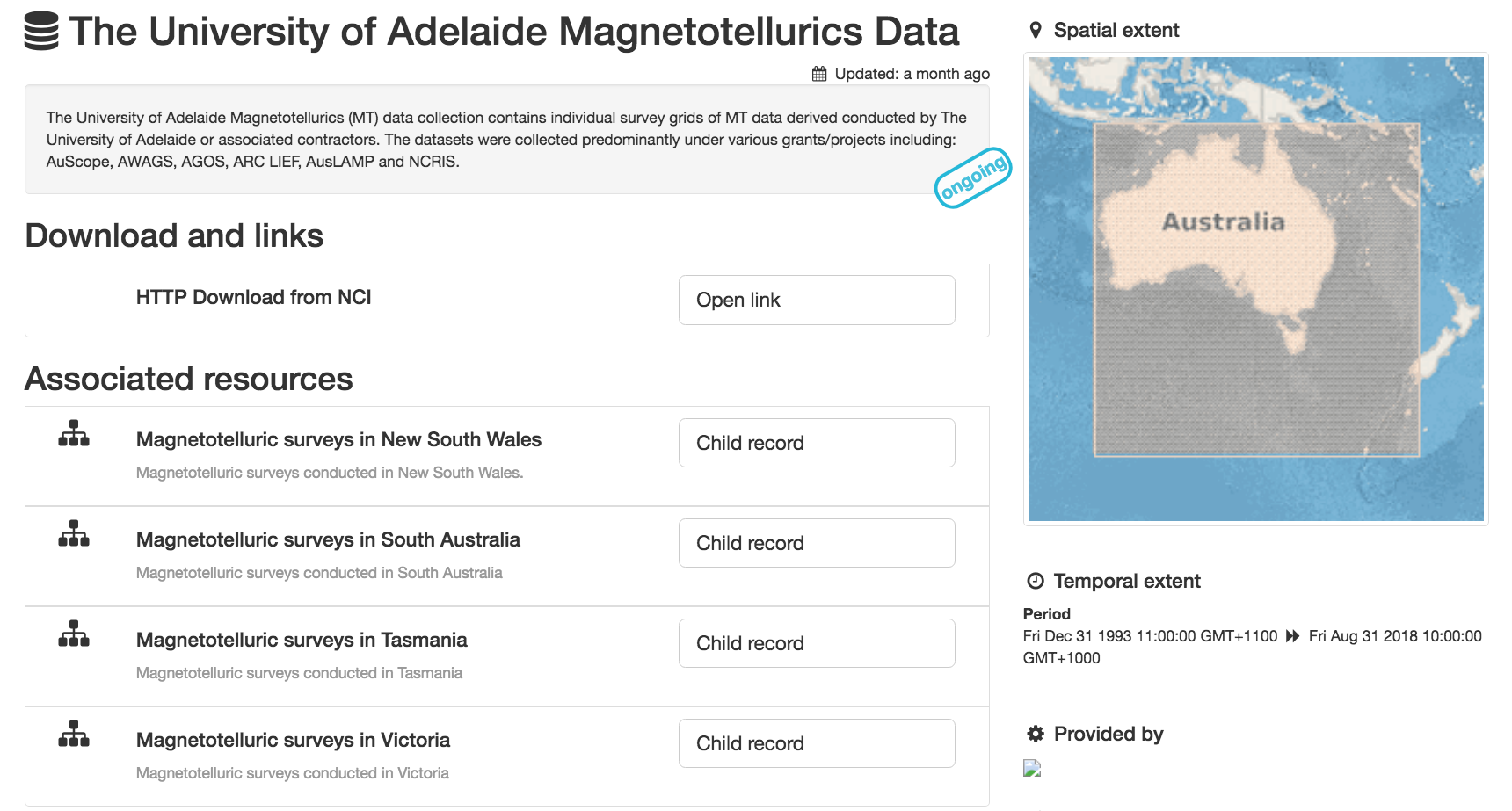
This page has a description of the parent record as well as links to the associated child resources.

Let’s take a look at the South Australia MT surveys:

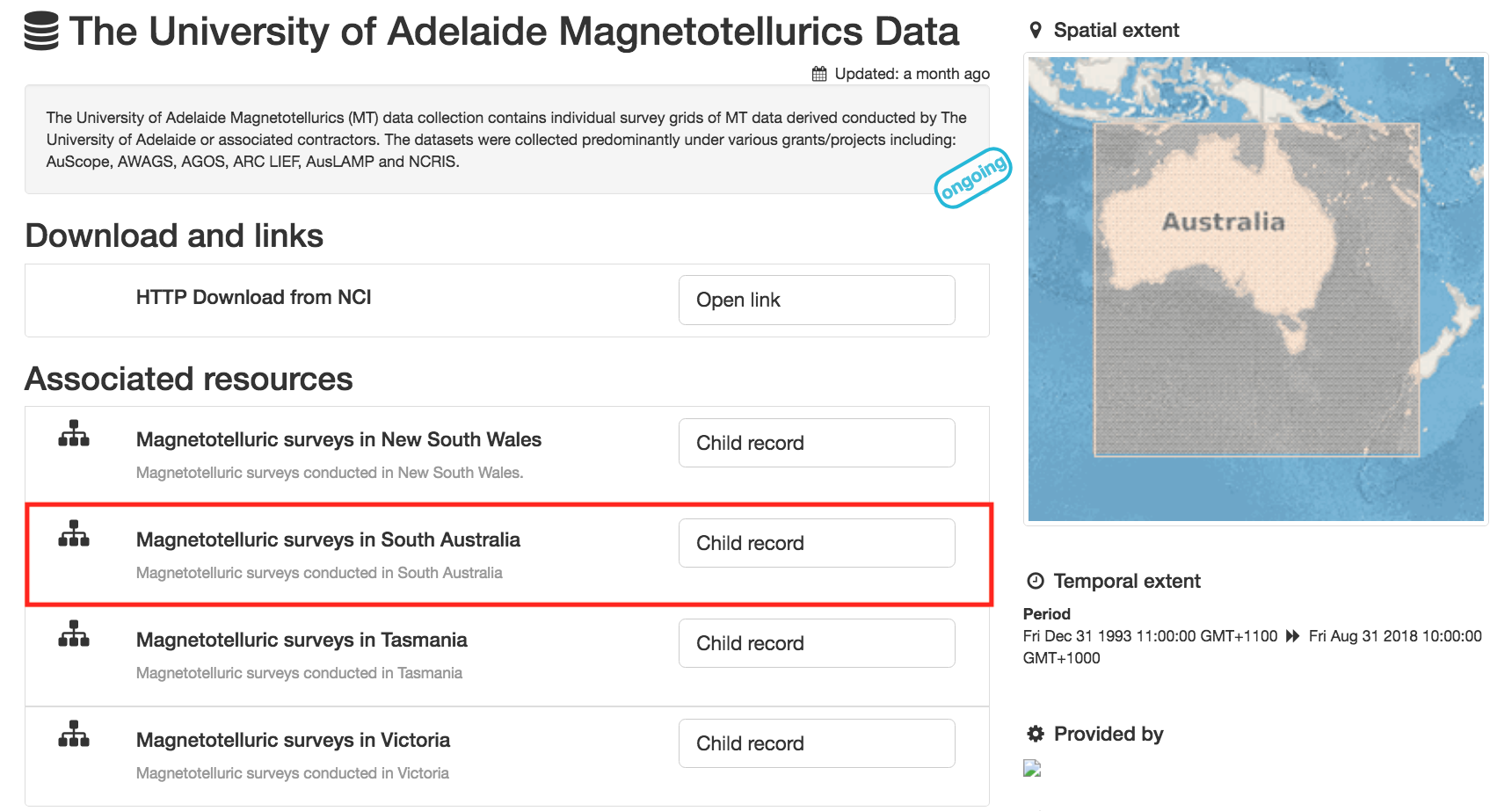
Here we can see a list of MT surveys conducted in South Australia

Let’s click on a survey of interest:

Here we can see:

an abstract describing the dataset
http download of the EDI files for this dataset
links to any papers or reference material associated with this dataset

MT software available at NCI¶

The following MT software:

are locally installed on NCI’s Raijin Supercomputer and Virtual Desktop Infrastructure (VDI) (currently under the project my80).

NOTE: To join the project my80, please log into mancini, click on the Projects and groups tab, then click on the Find project or group tab. Search for my80 and request to join.

Additionally, the seismogram browser Snuffler is available on NCI’s VDI.

BIRRP conditions of use:¶

1. The robust bounded influence magnetotelluric analysis program, hereinafter called BIRRP, is provided on a caveat emptor basis. The author of BIRRP is not responsible for or culpable in the event of errors in processing or interpretation resulting from use of this code.

2. No payment will be accepted by any user for data processing with BIRRP.

3. BIRRP will not be distributed to anyone. Interested persons should be referred to this website.

4. The author will be notified of any possible coding errors that are encountered.

5. The author will be informed of any improvements or additions that are made to BIRRP.

6. The use of BIRRP will be acknowledged in any publications and presentations that ensue.

ModEM conditions of use:¶

AUTHORS

Gary Egbert, Anna Kelbert & Naser Meqbel

College of Atmospheric and Oceanic Sciences

104 COAS Admin. Bldg.

Oregon State University

Corvallis, OR 97331-5503

E-mail: egbert@coas.oregonstate.edu

Fax: (541) 737-2064

Ph.: (541) 737-2947

http://www.coas.oregonstate.edu

COPYRIGHT

Both binary and source codes for the Modular Electromagnetic Inversion Software (hereafter ModEM) are copyrighted by The State of Oregon acting by and through the State Board of Higher Education on behalf of Oregon State University, an educational institution having offices at 312 Kerr Administration Building, Corvallis, Oregon 97331-2140 (hereafter, OSU) and ownership of all right, title and interest in and to the Software remains with OSU. By using or copying the ModEM, User agrees to abide by the terms of this Agreement.

NONCOMMERCIAL USE

OSU grants to you (hereafter, User) a royalty-free, nonexclusive right to execute, copy, modify and distribute both the binary and source code solely for academic, research and other similar noncommercial uses, subject to the following conditions:

1. User acknowledges that the Software is still in the development stage and that it is being supplied “as is,” without any support services from OSU. NEITHER OSU NOR THE AUTHORS MAKES ANY REPRESENTATIONS OR WARRANTIES, EXPRESS OR IMPLIED, INCLUDING, WITHOUT LIMITATION, ANY REPRESENTATIONS OR WARRANTIES OF THE MERCHANTABILITY OR FITNESS FOR ANY PARTICULAR PURPOSE, OR THAT THE APPLICATION OF THE SOFTWARE, WILL NOT INFRINGE ON ANY PATENTS OR OTHER PROPRIETARY RIGHTS OF OTHERS.

2. OSU shall not be held liable for direct, indirect, incidental or consequential damages arising from any claim by User or any third party with respect to uses allowed under this Agreement, or from any use of the Software.

3. User agrees to fully indemnify and hold harmless OSU and/or the Authors of the original work from and against any and all claims, demands, suits, losses, damages, costs and expenses arising out of the User’s use of the Software, including, without limitation, arising out of the User’s modification of the Software.

4. User may modify the Software and distribute that modified work to third parties provided that: (a) if posted separately, it clearly acknowledges that it contains material copyrighted by OSU (b) no charge is associated with such copies, (c) User agrees to notify OSU and the Authors of the distribution and provide copies of the modifications if requested, and (d) User clearly notifies secondary users that such modified work is not the original Software.

5. User agrees that OSU, the Authors of the original work and others may enjoy a royalty-free, non-exclusive license to use, copy, modify and redistribute these modifications to the Software made by the User and distributed to third parties as a derivative work under this agreement.

6. This agreement will terminate immediately upon User’s breach of, or non-compliance with, any of its terms. User may be held liable for any copyright infringement or the infringement of any other proprietary rights in the Software that is caused or facilitated by the User’s failure to abide by the terms of this agreement.

7. This Agreement shall be governed and construed in accordance with the laws of the State of Oregon.

COMMERCIAL USE

Any User wishing to make a COMMERCIAL USE of the Software must contact the lead author at egbert@coas.oregonstate.edu to arrange an appropriate license. Commercial use includes (1) use of the software for commercial purposes, including consulting or interpretation of geophysical datasets for fee; (2) integrating or incorporating all or part of the source code into a product for sale or license by, or on behalf of, User to third parties, or (3) distribution of the binary or source code to third parties for use with a commercial product sold or licensed by, or on behalf of, User.

MT software on Raijin¶

In order to use the Raijin MT software, let’s first login to Raijin:

$ ssh abc123@raijin.nci.org.au

where abc123 is your NCI username.

Now use a text editor (e.g. nano, emacs, vi) to edit your .bashrc:

$ nano ~/.bashrc

Add the following line to the bottom of your .bashrc:

$ export MODULEPATH=/g/data/my80/apps/modules/modulefiles:$MODULEPATH

Save and exit.

Run the following command in your terminal:

$ source ~/.bashrc

You should now be able to load the following MT modules:

$ module load birrp

$ module load occam1DCSEM

$ module load dipole1D

$ module load occam2D

$ module load mare2DEM

$ module load modem

Once these modules are loaded, to run BIRRP:

$ birrp-5.3.2

To test that BIRRP is working:

$ cd /g/data/my80/sandbox/capricorn_test

$ birrp-5.3.2 < CP1_LP_NR.script

To run OCCAM1DCSEM and/or DIPOLE1D:

$ occam1DCSEM

To test OCCAM1DCSEM is working:

$ cd /g/data/my80/sandbox/occam_test/occam1DCSEM/Canonical_RealImag_BxEyEz

$ occam1DCSEM startup

To run mare2DEM, we first need to load in the intel-mpi module:

$ module load intel-mpi

To run mare2DEM in inversion mode:

$ mpirun -np <number of processors> mare2DEM <input resistivity file>

To run mare2DEM in forward mode:

$ mpirun -np <number of processors> mare2DEM -F <input resistivity file>

To run mare2DEM in forward fields mode:

$ mpirun -np <number of processors> mare2DEM -FF <input resistivity file>

To test mare2DEM is working:

$ cd /g/data/my80/sandbox/mare2DEM/inversion_MT

$ mpirun -np 8 mare2DEM Demo.0.resistivity

To run OCCAM2D:

$ Occam2D

To test OCCAM2D is working:

$ cd /g/data/my80/sandbox/occam_test/Test2

$ Occam2D startup

To run ModEM:

$ mod2DMT

or

$ mod3DMT

Note: If you need to use the Mod3DMT_MPI parallel code, you will have join the group ModEM-geophys via the NCI Mancini page

Once you have access to this group, you can load in the following module:

$ module load ModEM-geophysics/2013.06

MT software on the NCI Virtual Desktop Infrastructure (VDI)¶

We can also access the MT software on the VDI. Once logged in to the VDI via Strudel (see the VDI user guide for installation instructions), open up a terminal and use a text editor (e.g. nano, emacs, vi) to edit your bashrc:

$ nano ~/.bashrc

Add the following line to the bottom of your bashrc:

$ export MODULEPATH=/g/data3/my80/apps/modules/modulefiles:$MODULEPATH

Save and exit.

Run the following command in the terminal:

$ source ~/.bashrc

Now you should be able to load in the following modules:

$ module load birrp

$ module load occam1DCSEM

$ module load dipole1D

$ module load occam2D

$ module load mare2DEM

$ module load modem

$ module load snuffler

BIRRP, OCCAM, mare2DEM and ModEM can be used as per the instructions for Raijin.

To run snuffler:

$ snuffler

Time-series QC using snuffler, a miniSEED time-series visualisation tool¶

The Snuffler is an interactive and extensible seismogram browser (but can also be used to view MT time-series) that is suited for small and very big datasets and archives.

For more information about Snuffler, please visit the Snuffler manual

For this example, we need to first log into NCI’s VDI. Once on the VDI, open up a terminal.

Let’s load in the module snuffler:

$ module load snuffler

For this example, let’s view some miniSEED data located here:

$ cd /g/data/my80/sandbox/snuffler_test/

To view this example time series:

$ snuffler *.mseed

and the following window should open:

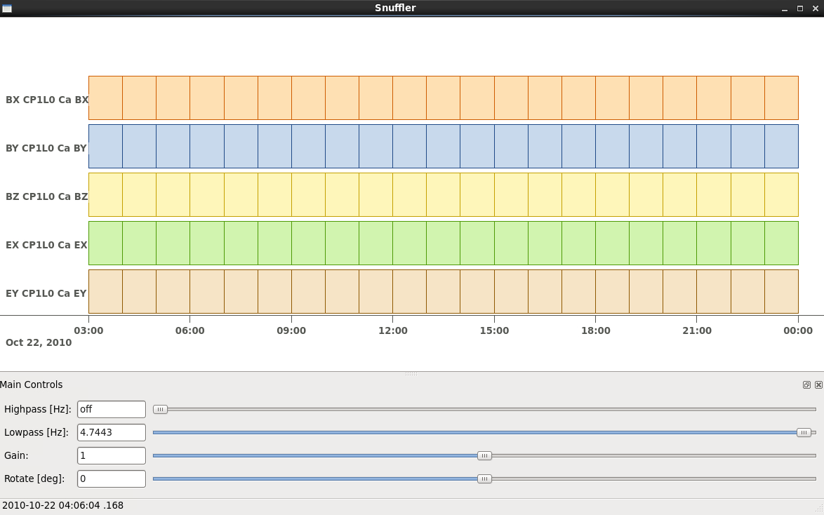
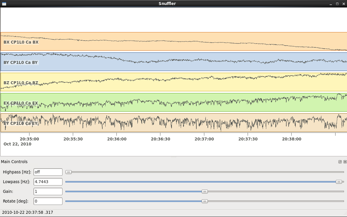
Initially there are no waveforms. To zoom in and view the waveforms, hold the mouse over the coloured boxes and pull towards you. Once you zoom in close enough, the time-series will appear. To zoom out, hold the mouse over the trace data and push the mouse away from you.

Navigation commands:

< space > - move forward one page in time

b - move backward one page in time

f - full screen is displayed

< minus > - remove one trace from the snuffler screen

< plus > - add a trace to the snuffler screen

: - toggle the snuffler command line

? - displays help information

For a more detailed look at how to use snuffler, please visit this snuffler tutorial.

Running the Bounded Influence, Remote Reference Processing (BIRRP) code on NCI’s VDI and Raijin¶

Once we are happy with the quality of our time-series, the next step is to run our time-series data processing. For this example, we will run the Bounded Influence, Remote Reference Processing (BIRRP) code of A.D. Chave and D.J. Thomsom.

For those unfamiliar, the BIRRP program computes magnetotelluric and geomagnetic depth sounding response functions using a bounded influence, remote reference method, along with an implementation of the jackknife to get error estimates on the result. It incorporates a method for controlling leverage points (i.e., magnetic field values which are statistically anomalous), includes the implementation of two stage processing which enables removal of outliers in both the local electric and magnetic field variables, and allows multiple remote reference sites to be used.

For more information about BIRRP and links to the relevant literature, please visit here

Using BIRRP on the VDI¶

A test dataset has been created with 16 MT sites and associated E/B time-series ready for BIRRP processing. Note that this test is mainly focusing on computational performance and not on the results of the BIRRP processing.

BIRRP script files for sites B1-B16 can be found here:

$ cd /g/data/my80/sandbox/capricorn_test/loop_test/

For example:

$ less B1/CP1.script

Let’s create a file with a simple loop to run BIRRP processing serially (one station after another) on each of our 16 MT sites. Run:

$ less serial_VDI.sh

to view the following script:

#!/bin/bash

for f in /g/data/my80/sandbox/capricorn_test/loop_test/B*;
  do
    [ -d $f ] && cd "$f" && echo Entering into $f and running BIRRP && birrp-5.3.2 < CP1.script && cd ..
  done;

To run this script:

source serial_VDI.sh

The job execution time for this script is approximately 30 minutes.

Now let’s slightly edit our script to run the 16 BIRRP executions in parallel using the 8 cores available on the VDI. Run:

$ less parallel_VDI.sh

to view the following script:

#!/bin/bash

for f in /g/data/my80/sandbox/capricorn_test/loop_test/B*;
  do
     [ -d $f ] && cd "$f" && echo Entering into $f and running BIRRP && birrp-5.3.2 < CP1.script && cd .. &

  done
  wait

To run this script:

$ source parallel_VDI.sh

The job execution time for this script is approximately 4 minutes.

Using BIRRP on Raijin¶

Let’s test our BIRRP processing script on Raijin using 16 cpus and 500MB of memory.

Login to raijin and run:

$ cd /g/data/my80/sandbox/capricorn_test/loop_test/

$ less parallel_VDI.sh

to view the following script:

#!/bin/bash

#PBS -P z00
#PBS -q normal
#PBS -l walltime=00:05:00
#PBS -l mem=500MB
#PBS -l jobfs=1GB
#PBS -l ncpus=16
#PBS -l software=birrp-5.3.2
#PBS -l wd

module purge
module load birrp/5.3.2

for f in /g/data/my80/sandbox/capricorn_test/loop_test/B*;
  do
     [ -d $f ] && cd "$f" && echo Entering into $f and running BIRRP && birrp-5.3.2 < CP1.script && cd .. &

  done
  wait

To run this script:

$ source parallel_raijin.sh

The job execution time for this script is approximately 1 minute.

Here we can see that by running our BIRRP loop on Raijin using multiple CPUs, we can significantly decrease our processing time. In theory we could run thousands of different BIRRP processes at once on Raijin. This same concept could be applied to running 2D inversions with OCCAM2D and Mod2DMT where one could run thousands of inversions in parallel by requesting the appropriate number of CPUs.

Installing and using MTpy on the VDI¶

MTpy: A Python Toolbox for Magnetotelluric (MT) Data Processing, Analysis, Modelling and Visualization

Written in Python, the code is open source, containing sub-packages and modules for various tasks within the standard MT data processing and handling scheme. For more information on MTpy, please read:

Krieger and Peacock 2014. MTpy: A Python toolbox for magnetotellurics. Computers & Geosciences, 72, 167-175.

We will now go through the installation of two versions of MTpy on the VDI:

V1: https://github.com/geophysics/mtpy

This is the original version of MTpy. The advantage of this version is it has few dependencies making it easy to install and use. This version will take up approximately 115MB of disk space.

$ cd ~/

$ git clone https://github.com/geophysics/mtpy.git

$ cd mtpy

$ python setup.py install

To test that mtpy has been installed:

$ module load python/2.7.11

$ module load ipython/4.2.0-py2.7

$ ipython

In [1]: from mtpy import utils

If this line of python code works then you have successfully installed MTpy on the VDI!

Now let’s try an example of converting BIRRP outputs to edi files. For this, we will work with an example BIRRP output found here:

/g/data/my80/sandbox/capricorn_test/loop_test/2M/M1/

Note that the BIRRP config file is CP1.script and the survey_configfile is survey.cfg.

Let’s head back to our ipython terminal

In [2] from mtpy.processing.birrp import convert2edi
In [3] stationname = 'c01'
In [4] survey_configfile = '/g/data/my80/sandbox/capricorn_test/loop_test/2M/M1/survey.cfg'
In [5] in_dir = '/g/data/my80/sandbox/capricorn_test/loop_test/2M/M1/'
In [6] birrp_configfile = '/g/data/my80/sandbox/capricorn_test/loop_test/2M/M1/CP1.script'
In [7] convert2edi(stationname, in_dir, survey_configfile, birrp_configfile, out_dir = None)

This should create the following edi file:

/g/data/my80/sandbox/capricorn_test/loop_test/2M/M1/C01.edi

V2: https://github.com/MTgeophysics/mtpy

This is the most up to date version of MTpy and will take up approximately 370MB of disk space. Additionally, a virtual environment needs to be created in order to install some of the dependencies, which will take up approximately 190 MB of disk space. This version of MTpy requires the following dependencies:

matplotlib>=2.02

numpy

PyYAML>=3.11

(geo)pandas

scipy

pillow

pyqt

qtpy

obspy

netcdf4

numpydoc>=0.7.0

To install:

$ cd ~/

$ git clone https://github.com/MTgeophysics/mtpy.git

Now we need to load in the required modules:

$ module load python/2.7.11

$ module load python/2.7.11-matplotlib

$ module load numpy/1.11.1-py2.7

$ module load scipy/0.17.1-py2.7

$ module load ipython/4.2.0-py2.7

$ module load pandas/0.18.1-py2.7

$ module load netcdf4-python/1.2.4-ncdf-4.3.3.1-py2.7

$ module load gdal/2.0.0

$ module load virtualenv/15.0.2-py2.7

and create a virtual environment::

  $ virtualenv mtpy_venv

  $ source mtpy_venv/bin/activate

Once the virtual environment has been activated, the following modules need to be installed via pip:

$ pip install pyyaml

$ pip install Pillow

$ pip install qtpy

$ pip install obspy

$ pip install numpydoc==0.7.0

Now we can install mtpy:

$ cd mtpy

$ python setup.py develop

To verify the install:

$ pip list | grep mtpy

To test, open up an ipython terminal:

In [1]: import mtpy.processing.birrp as birrp

If this works then MTpy has been successfully installed.

ModEM 3D inversions¶

Modular EM (ModEM) is a flexible electromagnetic modelling and inversion program written in Fortran 95.

It is currently available to use with 2D and 3D MT problems. For more information about ModEM, please read:

Kelbert, A., Meqbel, N., Egbert, G.D. and Tandon, K., 2014. ModEM: A modular system for inversion of electromagnetic geophysical data. Computers & Geosciences, 66, pp.40-53. - Kelbert et al. link

Egbert, G.D. and Kelbert, A., 2012. Computational recipes for electromagnetic inverse problems. Geophysical Journal International, 189(1), pp.251-267. - Egbert and Kelbert link

Let’s test the serial and parallel Mod3DMT codes on the VDI and Raijin for the ObliqueOne Inversion dataset given in the examples folder of the ModEM software.

Test 1: Serial Mod3dMT on the VDI

$ cd /g/data/my80/sandbox/modem_test/ObliqueOne/INV/

$ module load modem

$ mod3DMT -I NLCG  50_2x2_for_ObliqueOne.model Z_10_5_16p_100st_ObliqueOne_Noise50.data Inv_para.dat FWD_para.dat x02_y02_z02.cov

or

$ source my_script

The job execution time for this script was 1180m29s (almost 20 hours).

Test 2: Parallel Mod3dMT_MPI on Raijin

In order to use the Mod3DMT_MPI code, you will have join the group ModEM-geophys via NCI’s mancinipage. Once you have been granted access to this group:

$ cd /g/data/my80/sandbox/modem_test/ObliqueOne/INV3/

To run Mod3dMT_MPI, we need to create a shell script. For this example, let’s use the normal cue, 32 cups, 4GB memory and a walltime of 10 minutes:

#!/bin/bash

#PBS -P <project code>
#PBS -q normal
#PBS -l walltime=0:10:00,mem=4GB,ncpus=32,jobfs=100MB
#PBS -l wd

export OMP_NUM_THREADS=2

module load openmpi/1.10.2
module load intel-mkl/15.0.3.187
module load ModEM-geophysics/2013.06

mpirun -np 16 --map-by slot:PE=$OMP_NUM_THREADS /apps/ModEM-geophysics/2013.06/bin/Mod3DMT_MPI -I NLCG 50_2x2_for_ObliqueOne.model Z_10_5_16p_100st_ObliqueOne_Noise50.data Inv_para.dat FWD_para.dat x02_y02_z02.cov -v debug -P './tmpvec' > mod3dmt_oblique_test.out.$PBS_JOBID

To run this shell script:

$ qsub < mod3dmt_shell_script >

Experiment with some of the following commands to monitor the progress of this job:

$ qstat -u $USER

$ qstat -sw <jobID>

$ qstat -E <jobID1,...>

$ qstat -f <jobID>

$ qcat -s <jobID>

$ qcat -e <jobID>

$ qcat -o <jobID>

$ qls <jobID>

$ qcp <jobID>/* ./

$ qps <jobID>

$ nqstat_anu <jobID>

Once this job is complete, to see the stats:

$ qstat -u $USER -x

$ qstat -sw <jobID> -x

$ qstat -fx <jobID>

Additionally, 8 hours after the job is complete, the job stats should be available here

The job execution time for this script was 7m51s. For this example, using Mod3DMT_MPI on Raijin produces results almost 170 times faster than using the serial Mod3DMT on the VDI.

This material uses The University of Adelaide Magnetotellurics Data Collection which is available under the Creative Commons License 4.0.